
Code for this work can be found at https://github.com/Metric-Void/MPZ
Abstract
File Compression is an inherently serial task. Modern compression software utilities achieve some degree of parallelism by compressing multiple files simultaneously or dividing the input file into chunks and applying the same compression algorithm to all of them.
Our goal is to leverage higher levels of parallelism in order to achieve a higher compression ratio.
To take advantage of additional computation power, our algorithm tries different combinations of compression filters on different parts of the file. It then combines the results and selects the combination that results in the smallest output file size.
Our experiments show that our approach is effective at dividing and compressing various types of files and often outperforms the use of a single algorithm on the entire file, especially for heterogeneous files.
In this paper, we present two main contributions: 1) an investigation into the use of novel combinations of compression algorithms that achieve improved performance, and 2) a dynamic data chunking technique that allows for better fitting of compression algorithms on partitions of a large file.
Introduction
File compression is a powerful way of storing data with some degree of redundancy. For example, algorithms such as Huffman coding and arithmetic coding are effective at compressing files with uneven statistical distributions of characters. On the other hand, dictionary-based compression and referencing techniques can be used to compress repetitive data. Unfortunately, this process is inherently serial, as it involves examining the input sequence and storing references to previously encountered data in order to compress later data. As a result, it is difficult to utilize multiple threads or processes in the compression process.
Despite this, parallelism can be achieved by dividing the input data into several chunks and compressing each one individually. Many traditional algorithms took this approach. The zip utility, for example, will perform multi-threading when multiple files are being compressed; each thread focuses on compressing one file. Some archiving utilities achieve parallelism by dividing the input data into smaller chunks and doing them in parallel. For example, when asked to use multiple threads, the Linux XZ utility will read data into the memory, divide them into smaller chunks, and process them in parallel.
In this work, we aim to investigate the potential of compression if parallelism continues to grow. Traditionally, the approaches tend to divide the compressing targets into smaller chunks. However, dividing the input into smaller chunks will yield diminishing returns because the overhead for creating threads and distributing data will gradually exceed the time needed for compressing. Moreover, the lack of cross-reference among different chunks produces worse results as chunks get smaller.
We utilize the additional computation power by increasing the amount of work to be done. This approach is backed up by the fact that different compression algorithms target different kinds of data redundancy, and different algorithms perform differently on different types of files. If different compression algorithms are applied consecutively, they may generate either better or worse results, and the results also depend on the order they are applied. To fully utilize all available processors, we want our algorithm to explore different combinations of compression algorithms on different file chunks and draw the final result from all trials. Our approach will focus more on the compression ratio rather than compression speed.
In the final evaluation, we discovered that our program effectively divides the file at appropriate locations and generates smaller archives than using a single algorithm.
Related Works
Multiple prior approaches included the idea of combining various compression algorithms. The DEFLATE algorithm used for *.zip files, for example, is an algorithm that integrates LZ77 and Huffman coding. A more recent algorithm from Google, called Brotli, combines LZ77, Huffman coding, and second-order context modeling.
Our work focused on expanding parallelism by introducing more work that needs to be done. Traditionally, it is believed that permuting different sequences of compression filters and evaluating each will introduce a prohibitive computation cost because the effort needed is exponential to the number of algorithms to be tested. However, we observed that this computation cost could be offset with greater parallelism since each task is independent of others and can be distributed across multiple processes or machines. As a result, massively parallel computing systems allow one to find the best compression method within a reasonable time.
Background
This section reviews several commonly used and discussed compression algorithms and presents a brief explanation. These algorithms or their variations are included as the building blocks of our algorithm.
Huffman Coding. Huffman coding is an algorithm that encodes a sequence of symbols into a sequence of bits. It first analyzes the frequency of each symbol in the input and generates a variable-length prefix code for each symbol. Symbols that appear more frequently are given shorter coding patterns. Prefix codes are a set of bit patterns in which none of the patterns is the prefix of another, so no extra separation symbols are needed between each encoded symbol. A sequence encoded with prefix coding will not cause ambiguity when decoded.
Huffman Coding targets statistical redundancy in the data. Namely, symbols that appear more frequently are given shorter encoding patterns, so they do not take as many bits as in the original data. Symbols that appear less frequently might get bit sequences longer than their original encoding in the input, but the effect is more subtle since they do not appear as often.
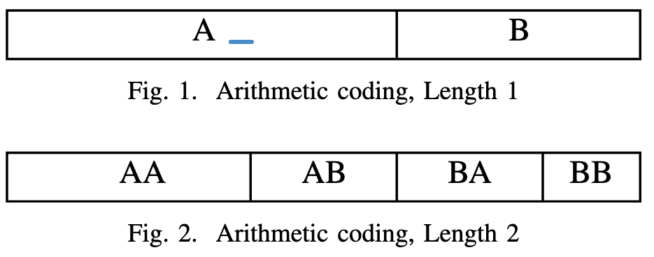
Arithmetic Coding. Similar to Huffman coding, Arithmetic coding also exploits the statistical distribution of symbol occurrences in the input sequence to compress data. It encodes a sequence of characters into a fractional number.
The encoding process works as follows: Assume we know the probability of character occurrences beforehand; say we have only two characters: A and B with probabilities pA and pB, with pA > pB and pA + pB = 1. The sequence A can therefore be encoded with any number in [0, pA), and the sequence B can be encoded with a number in [pA, 1), as shown in Figure 1. When more characters are added, these intervals are subdivided into smaller intervals. For example, AA can be any number in [0, pA × pA); AB can be any number in [pA × pA, pA); BA can be any number in [pA, pA + pB × pA); and BB can be any number in [pA + pB × pA, 1), as shown in Figure 2. Characters that appear more frequently will be assigned wider intervals. Therefore less significant digits are needed to represent such a sequence. The length of the encoded sequence is assumed to be known beforehand.
Arithmetic coding performs better than Huffman coding when the character set is small because it does not compress one datum at a time. For example, suppose the input sequence contained only (0, 1) as datums. In that case, Huffman coding will not be able to achieve any compression since it takes at least one bit to form the coding of each token, but arithmetic coding will work in this case.
Despite this fact, Huffman coding is much more ubiquitous than arithmetic coding in modern compression algorithms.
LZ77 and LZ78. Named after Abraham Lempel and Jacob Ziv, these two algorithms are two of the earliest dictionary-based compression algorithms published in 1977 and 1978, and the basis of many future dictionary-based compression algorithms. LZ77 reads the input data from the beginning and keeps a sliding window of previous sections. Repetitive data is replaced with a length-distance pair, which means "copy length bytes from distance bytes ago from the uncompressed stream."
The size of the sliding window limits LZ77’s compression ratio, and making the sliding window longer makes it slow. LZ78 attempted to solve this problem. In LZ78, all previously seen sequences are encoded as a trie (token tree). Each node is indexed with a number containing one token and a reference to its parent. A repeated sequence is encoded with the index of a node. When decoding, the sequence is reconstructed by tracing from that node back to the root of the tree to form a sequence of tokens.
LZMA is a combination of LZ77, and Markov Chains. It is an analog of Arithmetic Coding dictionaries, or range encoders, with a dictionary size of up to 4GB. Its compression speed is slow due to the large dictionary, but its decompression speed is on par with other algorithms.
Permutation Algorithms. Some character re-arranging techniques, such as Move-To-Front and Burrows-Wheeler Transform, can help reduce the entropy of the input data. Move-To-Front (MTF), for example, keeps a running list of the symbols, with the most recently used symbol moved to the beginning after each character is read. Each symbol in the input sequence is encoded as an index in the running list. If the input data tends to use similar symbols in a certain period, the generated sequence will contain more of smaller numbers, reducing entropy and benefiting other algorithms such as Huffman coding.
File-specific Algorithms. Some compression algorithms are designed specifically to compress one kind of file. For example, PACK200 is an algorithm specifically designed to compress and carry JAR files over the internet. It has methods specifically targeting Java byte code, acting like a compiler-level size optimization, and may produce slightly different files when decompressed. These types of algorithms are currently excluded from our consideration because our algorithm does not work on a per-file granularity, and this algorithm is not completely lossless.
Design
Parallelism
Our system is designed to run on the message-passing interface (MPI), with a master-worker orchestration model. A process with rank 0 will be the leader of this program, reading in the input stream and distributing jobs to different worker processes through MPI. Other programs, as workers, accept jobs, perform compression tasks and send results back to the leader. This approach allowed us to scale our algorithm across larger clusters, and it does not depend on maintaining a shared file system.
The input is fed into the leader program through an input pipe or a file. The leader will read the input stream in chunks, generate jobs that represent different computation patterns on this chunk, and send the jobs to the pool manager of workers. It then collects the results, compares which approach produced the best outcome, i.e., the smallest file size, and writes the processed chunk to the output file or stream in packets.
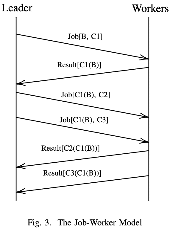
Figure 3 illustrates this procedure in a timeline. In this figure, B represents the original data, and C1, C2 and C3 are compression algorithms. The leader first asked a worker to apply C1 to the original data. After receiving the result C1(B), it then sends this result to available workers along with compress jobs C2 and C3 on this data, resulting in C3(C1(B)) and C2(C1(B)). This procedure will be repeated an adequate amount of times, and the leader will conclude the best result from all the executions.
Dynamic Input Chunking
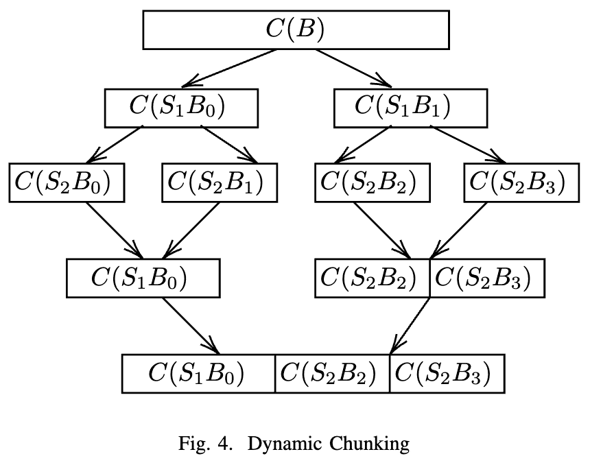
As mentioned in the previous section, the input is read in chunks. However, blindly dividing the input into chunks of the same size may cause inefficiencies. Although different parts of the file may have different patterns, chunks of the same fixed size are not likely to recognize good positions to separate the patterns and treat them differently. Therefore, we use a strategy similar to the Coding Tree Units (CTUs) in HEVC. Figure 4 illustrates our strategy: Each chunk is equally subdivided into two parts several times into smaller and smaller sub-chunks, denoted as SxBy in the figure, where x is the division level, and y is the sub-chunk ID. Different compression strategies will be applied to these smaller chunks, and check if the smaller chunks will be better compressed when being treated separately. For example, in Figure 4, the chunk B is recursively divided into smaller chunks until it reaches the smallest chunk size, shown as the second layer of the graph, S2B0 through S2B3. The results are then sent back to the recursion steps. On the left part of the tree, the recursion procedure handling sub-chunk S1B0 discovers that directly compressing S1B0 produces C(S1B0), which has a smaller size than C(S2B0) and C(S2B1) combined, so the leader chooses C(S1B0) as the final compression result of S1B0. On the right branch of the tree, the recursion procedure finds that C(S2B2)C(S2B3) has a smaller size than C(S1B1), so it chooses C(S2B2)C(S2B3) as the compression result of S1B1. This process propagates all the way back to the root of the tree, until which point we have the best way to divide the original chunk into sub-chunks and the compression result of the original chunk.
Search Space
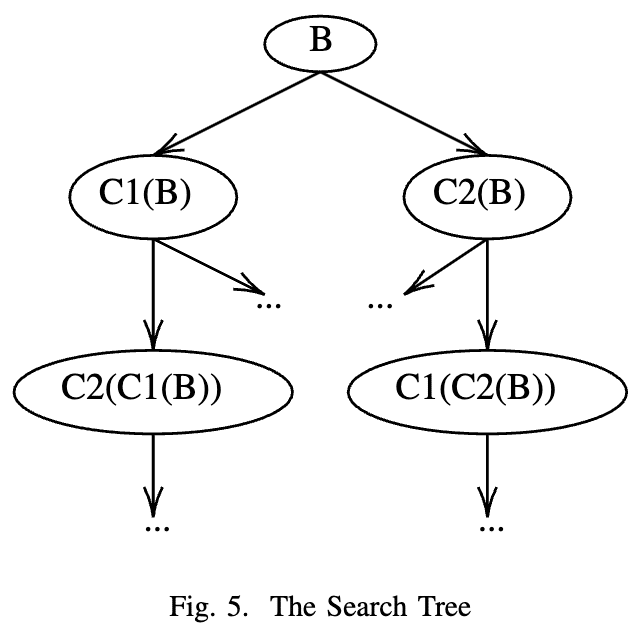
Figure 5 shows the search space of our algorithm. The B in this graph may either represent a raw chunk, or a sub-chunk produced by dynamic chunking as mentioned in the previous section. The search space is arranged in a tree structure, each edge represents a step of computation, and each node represents a result. After all the nodes are solved, the final step will collect all the results from all tree layers, and choose the one with the smallest compressed size. Each chunk/sub-chunk has its own search tree, and the leader will combine the best results.
In the ideal case, the tree should have a depth equalling the number of compression filters we have, exhausting all possible permutations. However, that would require computation and memory space on the order of O(NN), where N is the number of different compression filters. To reduce the search space, we observe that compression filters targeting the same type of redundancy will not be very effective if applied serially, so a search tree that’s excessively deep may not generate a better result. To limit the amount of calculation needed, we set the maximum depth of the search tree to two.
We included Move-To-Front, LZMA2, LZ4, BZIP, GZIP, and Huffman coding as the building blocks of the algorithms.
Output Data Format
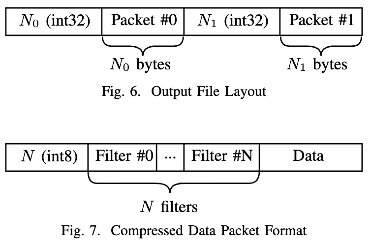
All kinds of compressed data and metadata are saved to the output file as a series of packets, as shown in Figure 6. The length of each packet is written to the output stream before the packet itself is written, making the packets separable.
We also considered another approach of using special marker symbols as the separator between packets. This method is employed by DEFLATE, which encodes some additional symbols (in addition to the 256 bytes 0x00 - 0xFF) into the Huffman tree and uses those pseudo-symbols as markers. That approach may save some space, but it requires the program to perform an additional step of histogram calculation and Huffman coding. Also, the decompression procedure must examine the input stream bit by bit on decompression so the packets can be separated. By comparison, the structure shown in Figure 3 allowed for parallel decompression. It does not take much effort for a thread to read, skip and distribute the packets. Each packet can be mapped to different workers and reduced back to the result, enabling some parallelism.
Figure 6 shows the packet format for compressed data. The first byte should be interpreted as a number, indicating the number of filters applied to the packet, followed by the IDs of the compression filters and, finally, the compressed data. When decompressing the data, the filters are decoded in reverse.
The packets will be written to a file output or the standard output stream. Since different chunks of the input file are processed in parallel, there must be a way to guarantee that the compressed data packets appear in the same order as they appear in the input stream. This is implemented by a buffered queue: The output file stream is managed by a singleton buffered output queue. Chunks at the master are managed by handles and assigned consecutive IDs. When these handles finish compressing the given chunk, they will send the resulting packets along with the ID to the output queue. When the queue receives packets with an ID that is consecutive to what it has previously written to the output, it will write that packet to the output right away. However, if packets with a later ID are received, the packet will be buffered and delivered when all previous packets are written.
Job dispatching
Job dispatching to the workers is conducted based on occupancy. The leader holds a dispatching queue for each worker, and the job will be queued to the worker with the shortest queue. If multiple workers have the shortest queue, a random one is selected. Round-robin does not apply to our case, since different compression algorithms take different times to finish, and round-robin may cause some inefficiency.
Communication Pattern
The communication pattern of our system is one-to-all. The leader process communicates with all the worker processes, and the workers do not communicate between them. When a worker completes the job, it will send the result back to the leader, and the leader will plan the downstream jobs and dispatch them. On the contrary, the leader process does no computation and focuses purely on moving data around. All computation is handled by the worker processes.
We also considered allowing worker-to-worker data transfers. On the surface, it may seem quite beneficial as the worker does not have to send the job result back to the leader. However, the search tree in Figure 5 requires O(N) jobs to be dispatched when each preceding job is completed, and sending the result back to the leader is just one additional message on top of that. This approach also creates difficulty in scheduling and dispatching jobs, since workers do not know which worker has the least occupancy, and workers may have difficulty figuring out where the result should be sent back to.
Threading Model
The leader process uses coroutines to manage workers efficiently. One coroutine is started at the leader process for each worker it manages, and only that coroutine is allowed to communicate with the worker, avoiding possible MPI message ordering problems.
Additionally, one coroutine is started for each chunk that needs to be processed. This coroutine schedules the jobs to the worker pool and waits for the result.
Although there seem to be a lot of coroutines, they will not slow the master process. Coroutines are very lightweight since they do not have memory specifically allocated for them like native threads. Also, these coroutines are suspended most of the time, waiting for results from workers.
Experiments
Inputs are fed into the program as tar archives, each tar file containing different kinds of files. The following datasets are benchmarked. It is worth mentioning that all file sizes presented here are estimations. The actual size of the files depends on what we find available on the Internet.
- 30MB of ASCII text file, crawled from English Wikipedia
- 16MB of UTF-8 e-Books fetched from the Gutenberg Project
- 32MB of pictures, fetched from unsplash.com
- 64MB of videos, fetched from pexels.com
- 32MB of binary Linux executable files, including gdb, vim, etc
- 32MB of randomly generated, IID bytes
- 16MB UTF-8 text file, 32MB pictures, 64MB videos, and 32MB of IID data
- 16MB UTF-8 text file, 32MB pictures, 32MB of Linux executable files
- 2MB UTF-8 text file, 8MB pictures, 4MB of UTF-8 text file, 8MB Linux executable files
- 183MB A PowerPoint presentation, with an embedded video and high-resolution pictures, fewer texts
- 153MB A PowerPoint presentation, with animations, pictures, and embedded data file for plotting
- 82MB A grayscale PDF e-Book in Chinese, with OCR characters
- 67MB RAW images from professional cameras
Experiments are conducted on an AWS machine with the OpenMPI library, with 2 sockets and 48 CPU cores of Xeon Platinum 8275CL. Since our focus is compression rate instead of execution time, the result is deterministic, and the execution environment is less relevant. During the period of this project, the Adroit cluster was highly occupied, and scheduling large jobs onto it gets a long slurm queueing time.
For all the experiments, the chunk sizes are set to 4MB, and the smallest sub-chunk size is set to 64KB. These values achieve a balance between compression performance and execution speed.
Results
All results presented here are extracted from the metrics file generated during compressing. The program logs the compression result of each chunk with each algorithm; an analyzer collects these results and constructs scenarios with and without each feature.
Practicality
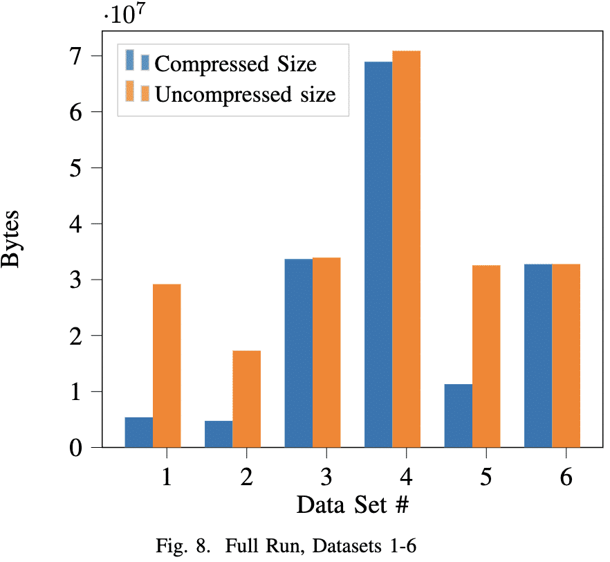
Figure 8 shows the result of our algorithm running on datasets 1 through 6. As conventional wisdom suggested, text files are compressed the best, followed by binary files, which may contain lots of similar opcodes and padding bytes. Videos and images barely compress. This result suggested that our program is capable of dealing with all kinds of data.
Adaptive Algorithms
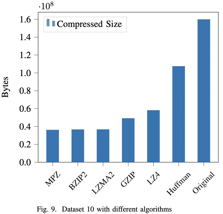
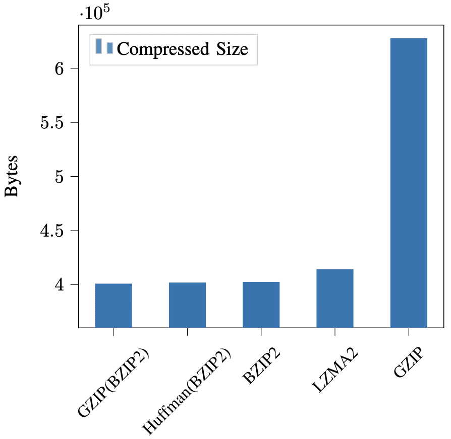
Figure 9 shows the effect of adaptive compression algorithm selection on the PowerPoint dataset 10. Our algorithm is shown as MPZ. By splitting the file into chunks compressed with different algorithms, we were able to achieve an archive file smaller than using any of them alone: 459,758 bytes of size reduction compared to using BZIP2 only, and 535,368 bytes smaller than using LZMA2 only. The logs files showed that our adaptive algorithm used GZIP, GZIP(BZIP2), straight Huffman, LZMA2, or leaving uncompressed.
Algorithm Chaining
Although our preliminary tests showed that some data gets compressed better when multiple algorithms are chained, the final results show that this is not very often. Figure 11 is the result of compressing a chunk of dataset 10, the PowerPoint presentation file. The combination of GZIP(BZIP2) scored the best result in *.pptx files multiple times but rarely performed better in other files.
GZIP implements the DEFLATE algorithm with LZ77 and Huffman coding. The specification of BZIP2 is incomplete; its document suggests that it’s a combination of the Burrows-Wheeler transform and Huffman coding, specifically optimized to compress text files. It is hard to explain why this specific combination of algorithms happened to be better. Still, it showed that our program has the potential to unveil algorithm combinations that perform better when chained.
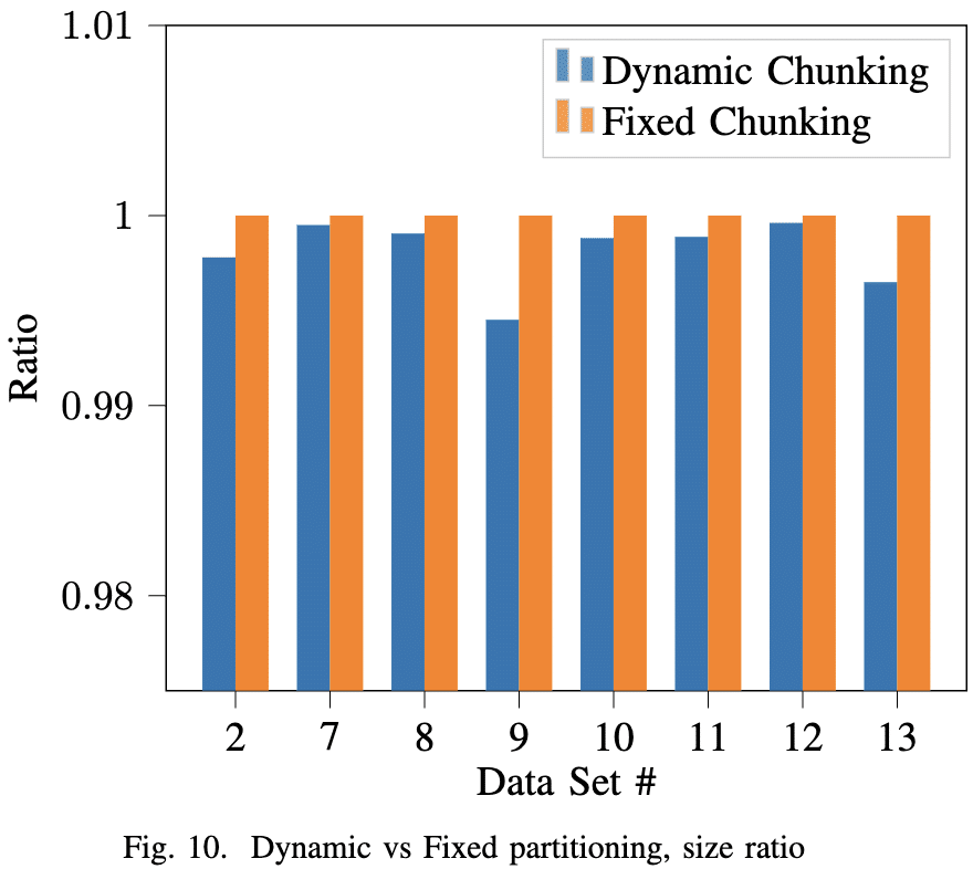
Dynamic Chunking
The smallest granularity of dynamic chunking is configurable in our program, with finer granularity leading to a deeper search tree and more computation.
Figure 10 shows the effect of dynamic chunking on our datasets. Its effect on the entire file is less significant - Around 0.05% in the best case. The benefit is highly dependent on the data patterns. The logs have shown that some chunks have a size reduction of 5.2%.
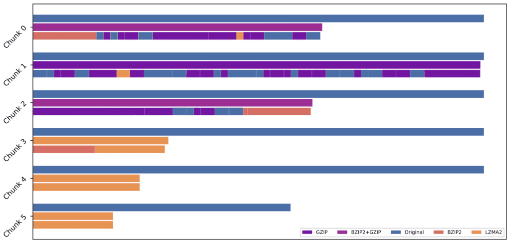
Figure 12 shows the layout of compressed dataset 9, with dynamic chunking, adaptive algorithm selection, and algorithm chaining. The file is divided into 5 chunks, and each chunk is displayed as a row in the graph. For each chunk, the first bar represents the original size, the second bar represents the size of the compressed chunk without dynamic input chunking, and the third bar represents the compressed chunk with dynamic chunking. Each algorithm used is rendered in a different color. As we can see, some parts of the data compress well with a single algorithm, while other parts of the file do not compress very well. Dataset 9 began with 2MB of UTF-8 text file, and our algorithm was able to determine that BZIP2 worked the best, the algorithm tailored for texts. 8MB of pictures following the text is barely compressible, and the algorithm struggled to find the best combination that made the file size the smallest. The program was also able to identify 4MB of text files spread across two different chunks, and finally, the 8MB of Linux executable files were compressed with LZMA.
Performance
Our program was able to occupy all the cores of our workstation fully. Compression is significantly slower than single approaches since it has to search many cases, but our algorithm was able to maximize its usage of system resources, and it took around 20 minutes to finish all the testing datasets on the workstation. We noticed that this algorithm takes up a huge amount of memory, approximately 8GB of memory per worker process. There is also an imbalance in resource consumption: Though the master process has roughly the same amount of CPU time as the workers, the master process takes up much more memory because it stores all the intermediate states and communication buffers.
Conclusion
We have implemented a parallel, MPI-based compression utility that utilizes parallelism to explore more possibilities on how the file can be compressed. Specifically, the algorithm will divide the file into various-sized chunks, try different algorithms, as well as combinations of algorithms on these chunks, and summarize the final result. From the results, our algorithm has proven that it can effectively search for algorithms, and the final compression ratio is better than using a single algorithm for the entire file. Moreover, our algorithm does not depend on the conventional wisdom of compression, making it a good candidate for discovering compression procedures that were previously not thought of.
Future Work
We propose several points that could demand some future work.
- Optimize for memory. The current approach takes a significant amount of memory and could cause some out-of-memory errors and get the process killed by Linux.
- Add more compression filters. The compression community is coming up with more and more algorithms for reducing the entropy of the input data, or compression algorithms that work well for a specific file pattern. Our algorithm can search for scenarios and combinations on when and where they work.
- Feature extraction can be added before compression algorithms are attempted on a chunk. A specific algorithm often has a favored data pattern, for example, the Huffman coding works better for data with small variance, so we can estimate the performance beforehand.
Comments NOTHING